The Evolution of Data Architecture

Every architectural decision Dataglot makes is a choice in a fifty-year argument. This essay explains the argument.

The modern data stack didn't appear from thin air. It is the cumulative answer to fifty years of mismatch between the questions people ask and the systems they had to ask them with. The relational database in 1970, the warehouse in 1994, the data lake in 2006, Snowflake in 2014, Iceberg in 2017, Arrow standardizing in-memory in 2016 — each was a response to a specific failure of the era before it.

The point is not to teach history for its own sake. It is that when someone says "let's just keep the cache layer simple," everyone in the room should understand what that simplifies away, what is lost by simplifying it, and which previous era's mistake would be repeated. Each chapter is a self-contained argument; read in order, they build the full mental model.

The story begins with the bundled relational database, the moment analytics broke it, the column-store answer, and the moment the internet broke that.

Chapter 1 — The original bargain (1970s)

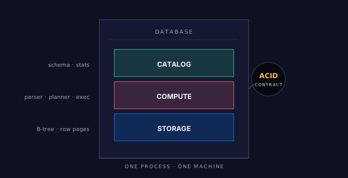
One process, one machine, one set of tables. Catalog, compute, and storage bundled together. The ACID contract was easy because everything happened in the same place at the same time.

The relational database, as Edgar Codd described it in 1970 and as IBM's System R and Berkeley's Ingres prototyped in the mid-1970s, was a complete world. The tables, the query engine, the transaction log, the indexes, and the access controls all lived inside a single trusted process running on a single machine. When a row was updated, the same process that knew about the table also wrote the change, also flushed the log, and also updated the index. There was no network boundary between any of these things, so there was nothing to coordinate, nothing to fail partway through, nothing to second-guess.

This is what made the ACID contract — atomicity, consistency, isolation, durability — feel almost trivial in the early systems. Atomicity ("all or nothing") is straightforward when there's only one writer. Consistency is straightforward when one process owns the schema. Isolation is straightforward when transactions are interleaved by a local lock manager. Durability is straightforward when the same process that holds the lock also fsyncs the log. The hard parts of ACID — distributed consensus, network partitions, partial failures — simply did not exist in the design space yet.

Storage was tuned for the dominant workload

The dominant workload was operational. Banks needed account balances. Airlines needed seat reservations. Retailers needed inventory levels. These were transactional questions: "show me row 12,847," "decrement quantity by one," "insert this transaction." The database engineers therefore tuned storage for that workload. Rows were laid out on disk together — all the columns of one record in one place. B-tree indexes made it cheap to find a row by primary key. The whole machine was an answer to "where is record N, and how do I update it safely?"

Year	Event
1970	Edgar Codd publishes "A Relational Model of Data for Large Shared Data Banks"
1974–79	System R (IBM Research) implements the first SQL prototype
1977	Oracle V2 ships — the first commercial relational database
1979	Ingres ships out of Berkeley
1980s	Sybase, Informix, DB2, Microsoft SQL Server

It is worth pausing on the shape of this system. Catalog, compute, and storage will reappear as separate, swappable layers in every architecture from the 2010s onward. In 1970, they are one rectangle. The history of the next fifty years is the story of that rectangle being pulled apart.

The bundled architecture worked because it matched the workload. Operational systems still look like this today — Postgres, MySQL, the embedded SQLite in your phone. The problem appeared when people started asking a different shape of question.

Chapter 2 — Then someone asked a different question

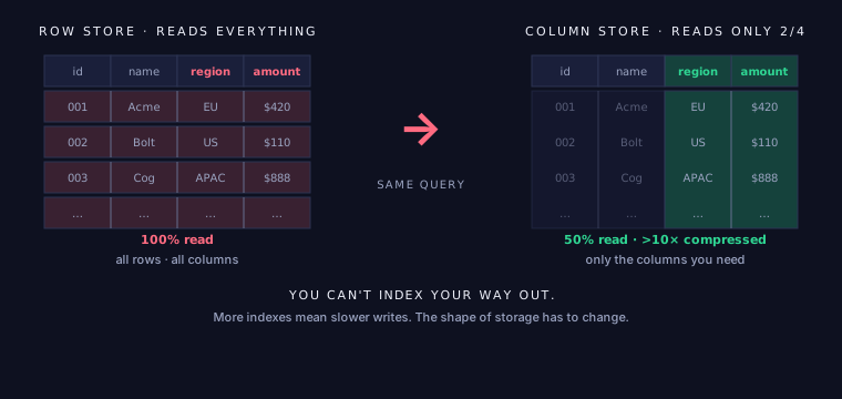
"Total revenue by region last quarter" needs only two columns out of forty. But row storage forces the database to read every full row from disk. The wasted I/O is the architecture, not a bug.

Sometime in the late 1980s and through the 1990s, businesses noticed that the same database that was running operations could in principle answer broader questions. Total revenue. Average order size. Trends across regions and quarters. These were not transactional questions about one row — they were aggregate questions over millions of rows.

When you tried to run them on the operational database, two things happened. First, the queries were unbearably slow. Second, while they ran, the operational workload slowed down too, because the analytics queries were holding shared resources and saturating the disks. The architecture that was perfect for "where is record N" turned out to be terrible for "summarize records 1 through N million."

The fundamental cost of the row layout

On a row store, every record is laid out on disk as a contiguous block of all its columns. To compute "total revenue by region," the database has to:

• Read each row of the orders table off disk, in full
• Throw away thirty-eight of the forty columns
• Keep the two columns that the query actually needs
• Repeat ten million times

The wasted I/O is not five percent or ten percent. For a forty-column table where two columns matter, the database is reading twenty times more bytes than it needs. Engineers called this read amplification — and it was the architecture, not a bug to be fixed.

It's tempting to suggest fixing this with indexes: just create an index on every column that gets queried. But indexes are not free. Every insert and every update has to rewrite every index that touches the changed columns. On a heavily-written operational table, indexing every analytical column kills write performance — which is the exact thing the operational database existed to do well. The architecture cannot serve both shapes of question.

This was the moment when the field forked. Operational systems would keep their row stores, B-trees, and tight transactions. A second species of system would emerge — purpose-built for analytics, with a different storage layout, a different query model, and a different posture toward data.

Chapter 3 — The pioneers turned the table ninety degrees (1994)

Sybase IQ shipped the first commercially-available column store in 1994. The trick was to lay out data column by column on disk. Reading two columns out of forty became cheap.

Instead of each row being a contiguous block of all its columns, each column was stored as a contiguous block of all its values. To answer "total revenue by region," the database now read only the bytes for the two relevant columns. Thirty-eight other columns stayed where they were on disk. Read amplification disappeared.

Sybase IQ was not the first columnar idea — academic systems and earlier work at Lockheed had explored it — but it was the first to ship as a productized, supported analytical database. The columnar idea later spread through MonetDB (1998, academic), C-Store (2005, the Stonebraker paper that became Vertica), and eventually into every modern analytical engine.

Three ideas, not just one

The data warehouse era introduced three distinct ideas, all of which still matter:

• Columnar storage — the layout itself, optimized for scans. Cheap to read few columns; cheap to compress within a column because all values share a type.
• MPP execution — massively parallel processing: partition the data across many machines, run the query in parallel, combine results. Teradata had been doing this since the early 1980s; the warehouse era productized it.
• Schema and modeling discipline — Ralph Kimball's dimensional modeling and Bill Inmon's normalized warehouse both became standard practice. The warehouse demanded that data be cleaned, conformed, and modeled before it was loaded.

That last point is what gave rise to the ETL industry. Data could not just appear in the warehouse — it had to be extracted from operational systems, transformed into the warehouse's schema, and loaded on a schedule. Tools like Informatica, DataStage, and Ab Initio were built specifically to run this nightly choreography.

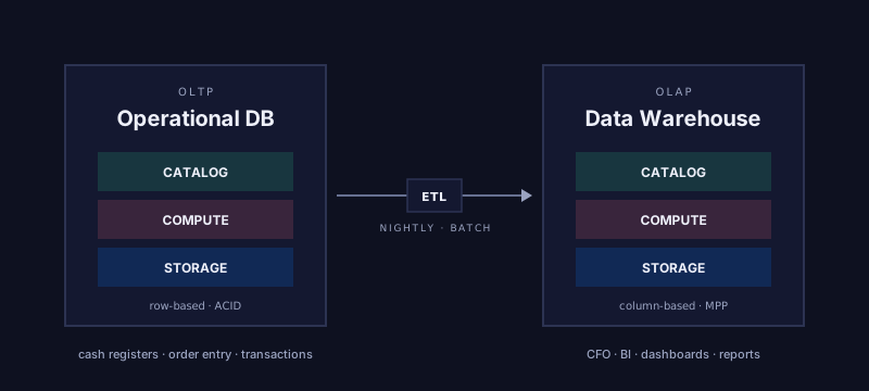
The architectural picture is now: two species of system, connected by a pipeline. Operational systems on the left, doing OLTP. Warehouses on the right, doing OLAP. ETL pipelines crossing the gap overnight. This was the dominant architecture for fifteen years, from roughly 1994 to 2010, and it is still how a lot of well-run analytical platforms work.

Year	Event
1979	Teradata founded — the first MPP analytical platform (shipped 1984)
1994	Sybase IQ ships — first commercial column store
1996	Ralph Kimball publishes The Data Warehouse Toolkit
1998	MonetDB (CWI Amsterdam) advances columnar academic work
2005	C-Store paper from Stonebraker et al. — basis for Vertica

The warehouse made analytics tractable, but it was an appliance. You bought the hardware and software together. Storage and compute scaled in lockstep. The data that could go in had to fit a schema you'd defined in advance. That last constraint is what broke next.

Chapter 4 — The internet broke the schema (mid-2000s)

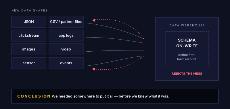
Web 2.0 pushed shapes the warehouse never expected through the door. JSON, web logs, clickstreams, video, sensor data. Schema-on-write meant the warehouse rejected anything it couldn't define up front — and most of the new data refused to define itself.

Through the early 2000s, the warehouse model assumed that data arrived in a known shape. Operational systems had defined schemas. ETL pipelines knew the source columns and the target columns. The warehouse could enforce types, foreign keys, and business rules at the moment data was written. This is called schema-on-write, and it was the warehouse's defining contract.

Then the web and mobile and IoT happened. Web server logs in idiosyncratic formats. Clickstreams with thousands of optional event types. Mobile app analytics where the schema changed every release. JSON documents from APIs that nested arbitrarily. Sensor readings at high frequencies. None of this fit cleanly into a relational schema, and even when it could be coerced, the schema would change weekly.

Three pressures at once

The warehouse couldn't hold the new shapes, but the bigger problem was that it shouldn't try. Three pressures hit simultaneously:

• Volume — clickstreams and logs were two or three orders of magnitude bigger than transactional data. A retailer's transactions might be 10 million a day; their clickstream might be 100 million events.
• Variety — data was no longer just rows. JSON documents, key-value pairs, time series, graphs. Some of it had loose structure; some had no structure at all.
• Velocity — the schema kept changing. Data engineers were being asked to ship a new column for the warehouse twice a week. Schema changes on a multi-petabyte warehouse were neither cheap nor reversible.

The famous "three Vs" framing of big data came out of this period. It was a polite way of saying: the warehouse is not the right tool for everything that is now data.

Engineering teams started keeping the new data on the side, in flat files on whatever storage they had — initially in HDFS, eventually in S3. The warehouse stayed for the structured analytical workloads it was good at. The new data lived elsewhere, with no schema enforcement, no transactions, and no real query engine on top of it. That accumulated pile of data would later get a name: the data lake.

The warehouse hadn't lost — it had run into a new requirement it was never designed to meet. What follows is how the field built a parallel infrastructure around the warehouse to handle the unstructured, the semi-structured, and the schema-changing — and how the rest of the modern stack is, in a sense, the long process of fixing that infrastructure's original sins.

Chapter 5 — S3 changed the economics (2006)

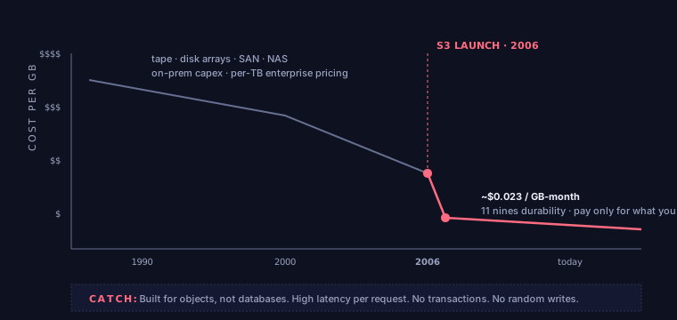
Object storage broke the economic constraint. "Keep everything" became a valid strategy for the first time in computing history. But cheap storage was not a database — high per-request latency, no transactions, no random writes.

In March 2006, Amazon Web Services launched S3 — Simple Storage Service. The pricing was startling. Fifteen cents per gigabyte per month at launch, dropping over time to fractions of a cent. There was no minimum, no provisioning, no upfront commitment. You PUT a file, you GET a file, you DELETE a file, and Amazon billed you for what you actually stored.

Compare this to the alternative. A traditional storage array required capital expenditure, capacity planning, and a storage administrator. A database that stored a petabyte required a hardware purchase that took months and was very hard to undo. S3 made storage so cheap and so elastic that, for the first time, the economically rational strategy was to keep all the data, indefinitely, regardless of whether you knew what you'd do with it later.

What "cheap storage" actually was

S3 wasn't a database. It was an HTTP API for storing and retrieving immutable blobs of bytes. Each object had a key, some bytes, some metadata, and that was it. There were no transactions, no indexes, no ability to update part of a file in place, and no native filesystem semantics. To "modify" a file, you uploaded a new version of the whole thing.

The properties were unfamiliar to anyone coming from databases:

• Eventually consistent (originally) — a PUT might not be visible to a GET on another machine for some seconds. Amazon fixed this in late 2020, but for the first fourteen years every system built on S3 had to handle eventual consistency explicitly.
• High per-request latency — a GET of a small file took tens to hundreds of milliseconds, not the microseconds of a local disk. IOPS were terrible compared to local SSD.
• High aggregate throughput — but if you read large objects in parallel, you got hundreds of megabytes per second per object, scaling linearly with concurrency.
• HTTP range requests — you could ask for just bytes 1000–2000 of an object instead of the whole thing. This turns out to matter enormously for what comes next.
• Effectively infinite — no capacity planning, no provisioning, no failed disks for the user to think about. Eleven nines of durability.

The mismatch with databases

These properties did not match what a database expects from storage. Databases assume small, fast, random-access I/O — the model of a local disk. S3 was the opposite: large, slow, immutable. A database that ran directly on S3 with no architectural changes would be unusably slow.

But the economics were so different that engineers were willing to redesign databases to fit S3, rather than the other way around. The next chapters are the story of that redesign. File formats had to change (Parquet). Engines had to change (Spark and the interactive SQL engines that followed). And eventually a new layer had to be invented above the files — the table format — because the lake by itself was not yet a database.

Year	Event
2003	Google File System paper (the inspiration for HDFS)
2006	Amazon S3 launches; Hadoop becomes a top-level Apache project
2008	Cloudera and Hortonworks form to commercialize Hadoop
2010	Azure Blob Storage, OpenStack Swift, Google Cloud Storage

S3 created the data lake by accident. It didn't intend to compete with databases. It just made storage so cheap that engineers started using it for everything, and the rest of the stack had to catch up. The catch-up took ten years.

Chapter 6 — Storage solved. Querying broken. (2006–2008)

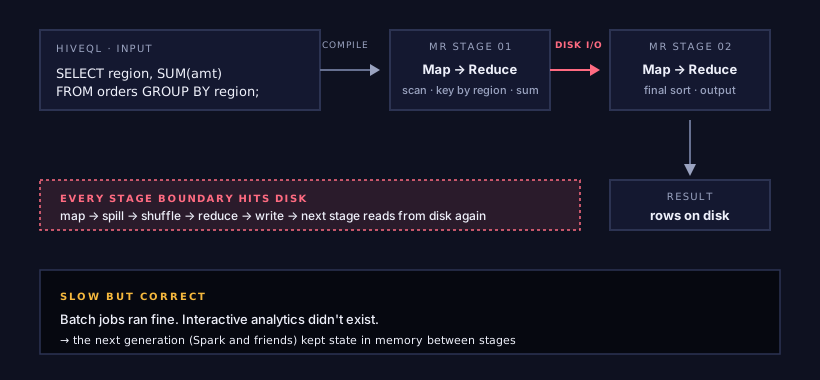
Hadoop and Hive gave analysts SQL on the lake. Under the hood, every query compiled into chains of MapReduce jobs that hit disk between every stage. It worked. It was not fast.

With cheap storage in place, the question became: how do we query this stuff? In 2006 Hadoop had emerged from Doug Cutting's work at Yahoo, implementing the ideas of Google's File System paper (2003) and the MapReduce paper (2004). HDFS gave you a place to put files. MapReduce gave you a way to run code over them. Together they were a usable, scalable batch processing platform — but only for engineers willing to write Java.

In 2008, Facebook released Hive. Hive translated SQL into chains of MapReduce jobs. An analyst could write SELECT region, SUM(amt) FROM orders GROUP BY region and Hive would compile that into one or more MapReduce stages, run them across the cluster, and return the result. SQL had arrived on the lake.

Why it was slow: disk between every stage

The MapReduce model had a fundamental performance ceiling. Every map phase wrote its output to local disk. Every reduce phase read its input from disk. If the query needed multiple stages — and most non-trivial queries did — each stage's output was written to disk before the next stage read it back. A query with three stages did three full disk-write-disk-read cycles. Even on fast disks, this dominated execution time.

The reason for the disk-between-stages design was fault tolerance. If a node died midway through a long-running job, MapReduce could restart just the affected task by re-reading its inputs from disk. This was a deliberate trade: correctness and resilience over speed. For overnight batch jobs on enormous datasets, that was the right trade. For analysts who wanted to iterate on queries interactively, it was unbearable.

What we lost relative to the warehouse

The Hadoop/Hive lake gave us scale and openness, but at the cost of nearly everything the warehouse provided:

• ACID semantics. Hive had no transactions worth the name. Concurrent writers could corrupt tables.
• Schema enforcement. Hive's metastore had a schema, but enforcing it depended on the writer's good behavior, not the system.
• Real indexing. Some bolt-on solutions existed, but the lake had nothing like the database's first-class index facilities.
• Interactive query latency. Even simple queries took seconds to minutes.
• Update and delete. The lake was append-only by design. Modifying rows required rewriting whole partitions.

Hive solved the access problem but exposed two new ones: the engine was too slow for interactive work, and the file formats it queried (text, CSV, sequence files) were terrible for analytics. Both got fixed over the next five years. Faster engines came first, but the file format work mattered more in the long run.

Chapter 7 — Columns came to the lake (2013)

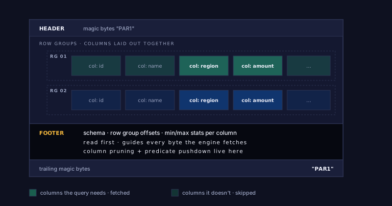
Parquet's anatomy is the answer to S3's physics. One self-describing file holds many row groups; each row group holds columns laid out together; the footer indexes everything. An engine reads the footer, decides which byte ranges to fetch, and skips the rest.

In 2013, Twitter and Cloudera jointly released Apache Parquet. The project drew its design from Google's Dremel paper (2010), which described how Google stored and queried nested data internally. Parquet brought columnar storage — the warehouse innovation from 1994 — to the data lake, in a file format that was open, language-agnostic, and tuned for object storage.

Parquet's importance is hard to overstate. It is the file format the entire modern lakehouse is built on. Iceberg tables, Snowflake external tables, DuckDB on S3 — they are all reading and writing the same Parquet files. The format won the way TCP/IP won: by being open, simple enough to implement everywhere, and good enough to defeat the alternatives.

Anatomy of a Parquet file

A Parquet file is a magic-byte header, followed by one or more row groups, followed by a footer (the metadata), followed by a closing magic byte. Each row group is a horizontal slice of the table — typically 128MB to 1GB worth of rows. Within a row group, the data is laid out column by column: all the values of column A first, then all the values of column B, and so on.

The footer is the trick. It holds the schema; the offset of every row group's every column chunk; per-column statistics (min, max, null count, row count) for every row group; and pointers to compression codecs and encodings. To answer a query, an engine first issues a small range request for the footer. Then it knows exactly which bytes hold the columns it needs, and issues parallel range requests for those bytes only. Everything else stays on S3.

This is what makes Parquet on S3 economically viable for analytics. Without the footer index, an engine would have to download whole files just to figure out what was in them. With the footer index plus column-grouped layout plus HTTP range requests, the engine downloads the minimum bytes needed.

Two query optimizations live in this layout

• Column pruning. The query needs columns A and C? Read only the byte ranges for A and C. Skip B, D, E.
• Predicate pushdown. The query has WHERE region = 'US'? Look at the per-row-group min/max statistics for the region column. If a row group's range is ['EU', 'EU'], skip it entirely — no rows in it can match.

Compression matters too. Within a column chunk, all values share a type, which makes compression dramatically more effective than on a row store. Parquet supports dictionary, run-length, and bit-packing encodings plus general-purpose compression (Snappy, Gzip, Zstd) on top. A typical Parquet file is 5–10x smaller than the same data in CSV.

Year	Event
2010	Google publishes the Dremel paper
2013	Twitter + Cloudera release Apache Parquet
2015	Parquet becomes a top-level Apache project
2016+	Universal adoption: Spark, Hive, Impala, Snowflake, BigQuery, DuckDB

Chapter 8 — The in-memory engines made it interactive (2010–2012)

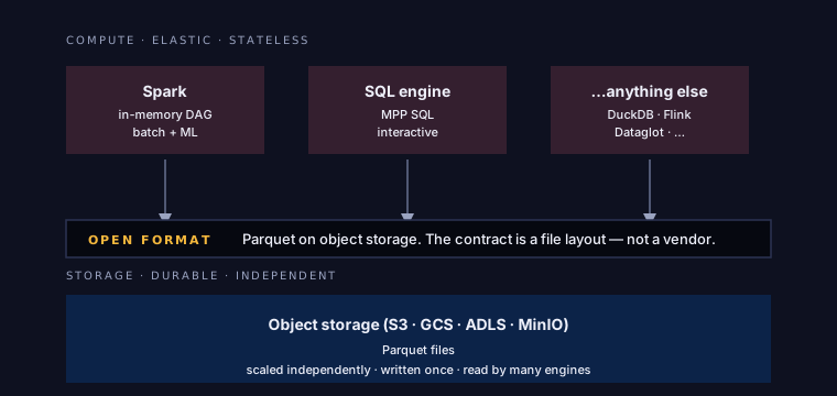
The new engines didn't own the data. They read open formats from object storage, computed in memory, and went away. Storage and compute scaled independently for the first time — a structural break from the appliance model.

Two engines fixed Hive's interactivity problem in the early 2010s. Both kept state in memory between stages instead of writing it to disk; both treated the storage layer as something they didn't own.

Apache Spark came out of UC Berkeley's AMPLab in 2009 and was open-sourced in 2010. Matei Zaharia's PhD thesis introduced the Resilient Distributed Dataset — a model where intermediate results stayed in memory across stages, with lineage tracked so lost partitions could be recomputed on failure. Where MapReduce hit disk between every stage, Spark hit disk only when memory ran out or the user explicitly asked.

A second wave of interactive SQL engines emerged inside the large web companies around 2012, designed from day one for ad-hoc analytical queries. They fetched data from many sources, computed in memory, and didn't persist anything between queries. A typical query that took ten minutes on Hive took ten seconds on this generation of engines.

The structural break: compute leaves storage behind

The deeper change wasn't performance. It was the relationship between compute and storage. In the warehouse era, compute and storage were bundled in a single appliance. In the Hive era, compute and storage ran on the same physical cluster, even though they were different software layers.

Spark and the interactive engines broke that. They read data from wherever — HDFS, S3, a JDBC source, a Kafka topic — computed over it in their own process, and returned results. The storage layer didn't know the engine existed. The engine didn't own the storage. They communicated through an open file format (often Parquet by this point) and an object-storage API.

The "thin wire" between compute and storage is, in practice, a file format spec plus an object-storage API. As long as an engine can read Parquet and speak S3, it can join the party. This is what lets Spark, DuckDB, Snowflake, and every engine since operate on the same files — and it is the architectural pattern the rest of the modern stack inherited.

Independent scaling

Decoupling compute from storage had an operational consequence: they could be scaled independently. Need to run a very large query? Spin up more compute for an hour. Data grew? Only storage scales. This had not been true of the warehouse era, where buying more storage meant buying more boxes with more compute attached, whether or not you needed it.

Year	Event
2009	Spark prototyped at Berkeley AMPLab
2010	Spark open-sourced
2012	Interactive SQL engines emerge inside the large web companies
2013	Spark becomes an Apache top-level project

Once compute and storage came apart, the question was no longer "which appliance?" but "which engine, on which storage, for which workload?" That question is still being answered — and it is the question Dataglot exists to answer well: an engine that speaks the same open formats can be adopted without migrating any data.

The lake now had cheap storage, good files, and fast engines. What it didn't have was a real table.

Chapter 9 — Snowflake separated everything (2014)

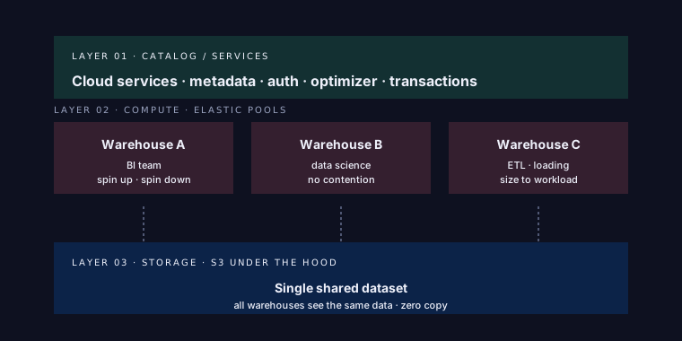
Snowflake (general availability 2014) made the three-layer separation a commercial product. Storage in S3, compute as elastic warehouses, services and metadata as a managed layer. The warehouse re-emerged in cloud form — proving the model worked at scale.

Snowflake's first beta was 2012; general availability was 2014. The architecture was unusual at the time. Storage was Amazon S3. Compute was "virtual warehouses" — clusters that customers could spin up, resize, suspend, and clone independently. The catalog and metadata services were a Snowflake-managed layer that all the warehouses talked to. These three pieces — storage, compute, services — could each be scaled, billed, and operated independently.

From a customer's point of view, this was magic. You could leave the data in place, spin up a "small" warehouse for a regular reporting workload and a "4XL" warehouse for a one-off analytical job, and have them both reading the same tables at the same time without contention. Storage cost almost nothing. Compute cost what you used and nothing else.

What Snowflake proved

Snowflake's commercial success — IPO in 2020 at one of the largest software valuations in history — proved several things that mattered architecturally:

• The three-layer separation worked at scale. Customers ran serious workloads. The architecture wasn't a curiosity; it was production-grade.
• Object storage was good enough. Snowflake stored the underlying data in S3 (or equivalents). The latency penalty was manageable; the economics were unbeatable.
• The catalog was the lock-in. Snowflake's storage format was proprietary; customers couldn't take their data and run it through someone else's engine. The metadata, the optimizer, and the SQL layer were where Snowflake earned its margin.

That last point matters for what comes next. Snowflake had separated storage, compute, and catalog architecturally — but kept all three under one vendor's roof. This was acceptable in 2014 because the alternative — running and tuning your own warehouse — was much worse. But it left a strategic opening. If the same three-layer separation could work with open specs at every layer, customers could keep their data on their own storage, in an open format, and choose the engine they wanted on top. That was the next architectural move.

Year	Event
2012	Snowflake founded; Amazon Redshift launches
2014	Snowflake reaches general availability
2017	Google BigQuery becomes broadly adopted
2020	Snowflake IPO

Chapter 10 — A pile of files is not a table (~2014–2016)

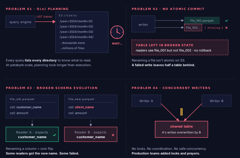
The lake had cheap storage, good files, fast engines. What it didn't have was a real table. The Hive Metastore tried — and broke at petabyte scale.

By 2014, the open lake had three of the four layers it needed. What was missing was a coordination layer that would turn a directory of Parquet files into something that behaved like a table — atomic transactions, schema evolution, time travel, safe concurrent writers.

The placeholder was the Hive Metastore, built in 2008 as a relational database tracking Hive's tables and partitions. It worked well enough for Hive's batch workloads. As people started running Spark and other engines against the same data, and as table sizes grew into the petabyte range, its limits became failure modes.

The four failure modes

O(n) query planning. The metastore tracked tables and partitions, but not individual files. To plan a query, the engine had to list the relevant directories on S3. At petabyte scale, with hundreds of thousands of partitions and millions of files, the LIST calls themselves became a major fraction of query time. Some queries spent more time planning than executing.

No atomic commits. S3 has no native rename. To "atomically" replace a file, the convention was write-then-rename — but S3 rename is copy-then-delete, two separate operations that can fail in the middle. A failed write left the table in a state where some new files were visible and others were missing. Readers saw partial results. There was no rollback because there was no concept of a transaction.

No safe schema evolution. Hive resolved column references by name. If a column was renamed, files written before the rename had the old name and files written after had the new one. Some readers got the new name. Some failed. Some silently returned wrong results.

Concurrent writers corrupt. With multiple engines writing to the same table, there was no coordination protocol. Two writers could overlap, one's changes could overwrite the other's, and the metastore had no way to detect it. Production teams added external locking with Zookeeper or by convention. Convention failed. Locking was fragile.

Each individual problem had workarounds. Each workaround was complicated. Together they meant that running the lake at scale required a small team of specialists watching the system constantly. This is not what a "table" is supposed to require.

Netflix's team did exactly this in 2017.

Chapter 11 — Netflix turned files into tables (2017)

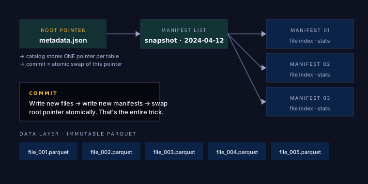
The whole table — every snapshot, every file, every statistic — is reachable from a single root pointer. A commit is a swap of that pointer. That's how Iceberg makes ACID transactions on a pile of immutable files.

Ryan Blue and Daniel Weeks at Netflix started designing what became Apache Iceberg in 2017. Netflix had hit every Hive Metastore failure at production scale. They built an alternative, open-sourced it in 2018, and donated it to Apache, where it became a top-level project in 2020.

Iceberg's design is conceptually simple: store the entire description of a table in a tree of metadata files in object storage, with a single root pointer at the top. To commit a change, write new metadata files describing the new state, then atomically swap the root pointer. Old metadata stays where it was — you can read older versions of the table just by pointing at older roots. This one mechanism gives Iceberg time travel, rollback, and snapshot isolation.

The metadata hierarchy

Walk the tree top-down:

• Root pointer — a single file (typically metadata.json) that names the current snapshot. The catalog stores this pointer. A commit is an atomic swap of which file the catalog points at.
• Manifest list — for the current snapshot, the list of all manifest files plus partition-level statistics.
• Manifest file — an index of data files, with per-file statistics: column min/max, null counts, row counts. This is what lets Iceberg plan queries in O(1) without listing S3 directories.
• Data files — the actual Parquet files. Immutable. Updates work by writing new data files plus delete files; the old data stays where it is, which is what makes time travel and rollback work.

How each Hive failure gets fixed

• O(n) planning becomes O(1). The engine reads one metadata file and follows pointers, instead of listing thousands of S3 directories.
• Atomic commits work via pointer swap. The catalog's update of the root pointer is a single atomic operation — either it happened or it didn't. No half-states.
• Schema evolution works on column IDs, not names. Iceberg assigns each column a stable numeric ID at creation. Renaming a column changes the name in metadata but not the ID. Readers reference the ID and find the data correctly across versions.
• Concurrent writers are serialized. Two writers each prepare their new metadata and both attempt to swap the root pointer. The catalog's atomic compare-and-swap lets exactly one win. The loser retries against the new state. No corruption, no locks.

What snapshot isolation gives you for free

Because old metadata is kept until explicitly expired, readers always read against one consistent snapshot. While a writer commits, in-flight readers continue reading the previous snapshot, uninterrupted. Time travel and rollback fall out the same way: want the table as it was last Tuesday? Read against that snapshot. Want to undo a bad write? Swap the root pointer back. These features are not bolted on — they are inherent in keeping snapshots around.

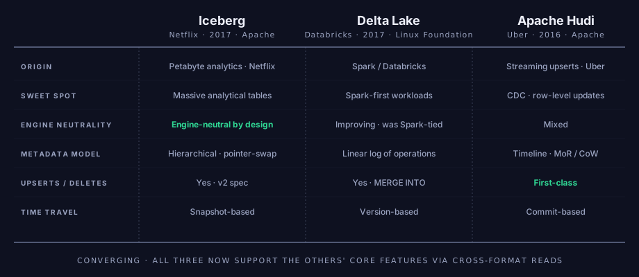
Two competing table formats appeared around the same time. Delta Lake (Databricks, 2017) was Spark-first by design, with a transaction-log-based metadata model. Apache Hudi (Uber, 2016) was streaming-first, optimized for row-level upserts and CDC. All three now solve roughly the same problems with different bets, and they have been converging — but Iceberg has the broadest multi-vendor adoption (Snowflake, Spark, DuckDB, Athena, BigQuery all read it) and the most engine-neutral design philosophy.

Year	Event
2017	Design starts at Netflix
2018	Open-sourced; donated to Apache
2020	Top-level Apache project
2024	Snowflake announces support; Databricks acquires Tabular; de facto standard for the open lakehouse

Iceberg is the keystone of the modern open lakehouse. Dataglot is built to be a first-class Iceberg engine — it reads and writes Iceberg tables natively, with no proprietary intermediate format anywhere.

Chapter 12 — Arrow, the connective tissue (2016)

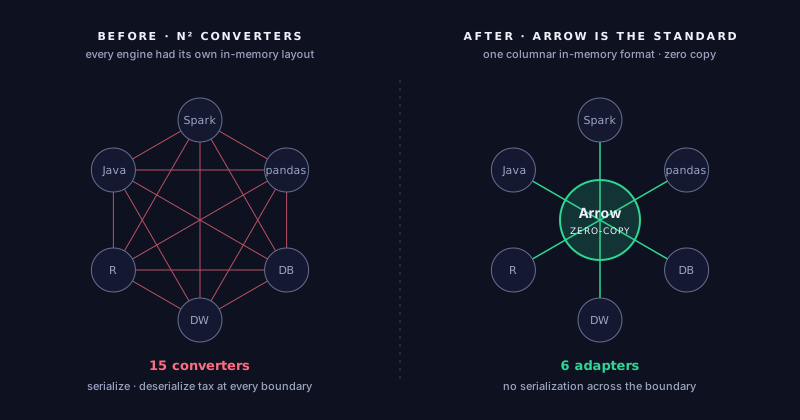
Every engine had its own in-memory layout. Crossing from Spark to pandas to a database meant constant serialization. With N systems, you needed N² converters. Arrow standardized the in-memory format itself.

A historical note on order: Arrow was open-sourced in 2016, before Iceberg's 2017 design. It belongs here in the narrative because it is best understood as the in-memory complement to Parquet's on-disk story. Parquet standardized the columnar layout on disk; Arrow standardized the columnar layout in memory. Together they let data move through the modern stack without conversion taxes at any layer.

Apache Arrow was started by Wes McKinney (creator of pandas) and Jacques Nadeau (Drill, Dremio) along with collaborators from across the analytical ecosystem. The project's defining commitment is a precise, language-agnostic specification of how columnar data is laid out in RAM. Once two systems both implement the spec, they can share data without copying or transforming it — even when they're written in different languages.

The N² problem Arrow solved

Before Arrow, every analytical engine had its own in-memory representation. Spark had Project Tungsten's binary format. pandas had NumPy-backed columns. Drill had value vectors. When data moved between systems — a Spark job feeding a pandas analysis, a SQL engine's result feeding a Python ML model — every boundary required serialization on one side and deserialization on the other.

With N different systems, the ecosystem was building roughly N² conversion paths. Worse, serialization is not free: at scale, the conversion CPU and memory cost dominated end-to-end time. Some workloads spent more time converting between formats than computing.

Arrow inverts the topology. Every system implements the Arrow spec; conversions happen at the edges of each system, not at every pair. With 6 systems, you need 6 implementations, not 15 converter paths. And because the in-memory layout is identical across systems, two processes can share the same memory pages directly — zero-copy. The bytes don't need to be touched at all.

Arrow Flight: the wire protocol

Beyond the in-memory format, the project ships Arrow Flight — a wire protocol for moving Arrow batches over the network. Flight replaces row-by-row protocols like ODBC and JDBC with columnar batches over gRPC. For analytical workloads that move millions of rows, this is dramatically more efficient — orders of magnitude in some benchmarks.

Why this matters for Dataglot

Dataglot is Arrow-native end to end. Connectors return Arrow batches. The execution engine runs over Arrow. Results leave the system as Arrow. There is no internal serialization tax — which matters most in federation, where data crosses many source and process boundaries on its way to one result set.

Year	Event
2015	Wes McKinney and Jacques Nadeau begin discussions
2016	Apache Arrow announced
2018	Arrow Flight introduced
2020+	Adoption across pandas, Spark, BigQuery, Snowflake, DuckDB, DataFusion, ClickHouse

If Parquet and Iceberg are the open contracts on disk, Arrow is the open contract in RAM. The last two chapters put all six layers together — and walk through where Dataglot builds on each one.

Chapter 13 — The stack converged

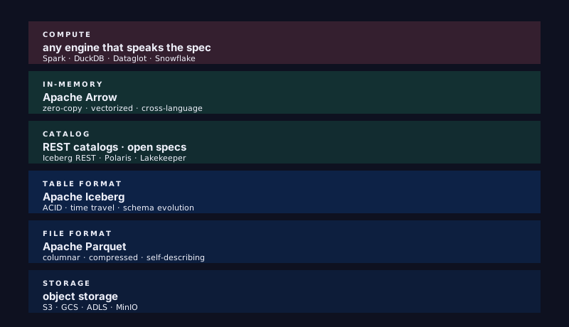
A layered, spec-driven stack. Each layer is independently swappable. Storage and compute scale separately. Catalogs are open. Engines compete on execution quality, not data lock-in.

The cumulative result of the history is the modern open lakehouse: a six-layer stack where every layer has an open specification and every layer can be replaced without rewriting the others.

The six layers, top to bottom

Read them top to bottom. Each layer's job is to make the layer above it work without owning the data.

Layer	What lives there
Compute	The query engines: Spark, DuckDB, Dataglot, and the rest. Each speaks the open specs below. Stateless and elastic — spin up for a query, spin down. Engines compete on execution quality, not on owning your data.
In-memory	Apache Arrow. The columnar byte layout every engine reads and writes. Zero-copy across language boundaries. Eliminates the serialization tax at engine handoffs.
Catalog	The transactional table directory. The Iceberg REST catalog spec lets multiple engines safely share the same tables. Polaris and Lakekeeper are open implementations.
Table format	Apache Iceberg (plus Delta Lake and Hudi for specific workloads). Turns a pile of immutable files into a transactional, time-traveling, schema-evolving table.
File format	Apache Parquet, near-universally. Self-describing columnar files with a footer index, optimized for object storage via byte-range requests.
Storage	Object storage: S3, GCS, ADLS, MinIO for self-hosted. Cheap, durable, infinite. The same Parquet files can live on any of them — you can change vendor without rewriting data.

The structural insight

Look back at chapter 1. In 1970, all six layers were one rectangle — a single process that owned the tables, the engine, the log, and the access controls. Today, all six layers are separate, swappable, and governed by open specs. That progression — from a single bundled appliance to six independently-replaceable layers — is the entire fifty-year argument.

The architectural point of the lakehouse isn't just "open formats." It is that every layer is replaceable independently. You can change your engine without touching your data. You can change your storage without touching your engine. You can change your catalog without rewriting either. This is what eliminates lock-in — not openness in any one place, but the systematic decoupling of every layer from every other.

Where the competitive battle is

With the lower layers (storage, files, table format) commoditized, the competitive question moves up. Two layers are still genuinely contested:

• The compute layer — engines compete on execution quality, on which workloads they're best at, on developer experience.
• The catalog layer — semantic metadata, governance, multi-tenancy, business meaning. The catalog wraps the table format and adds the things that turn raw tables into a usable platform.

Dataglot competes in the compute layer — with governance enforcement as a first-class engine capability rather than an add-on that wraps the engine.

Chapter 14 — Why Dataglot

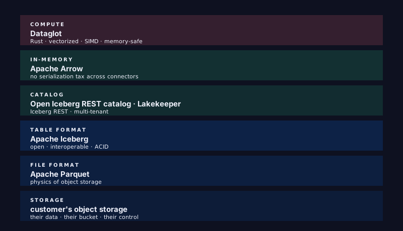
Same six layers. Specific choices at each one. Every decision is defensible by pointing back at the chapter that motivated it. There are no surprises.

Compute — Dataglot itself

Built in Rust: vectorized, SIMD-aware execution with memory safety guaranteed by the language. What that buys you is an engine that starts in milliseconds, ships as one static binary, and doesn't carry a JVM's memory ceremony or garbage-collection pauses into your query latencies — and an engine that doesn't segfault is an engine you can trust with production credentials. Under the hood it builds on proven Apache foundations (DataFusion for query execution) rather than reinventing them. (See chapter 8 on why fast vectorized engines matter, and chapter 12 on Arrow as the in-memory currency.)

In-memory — Apache Arrow

Native end to end. Connectors return Arrow batches. Execution stays Arrow. Results leave as Arrow. No internal serialization tax — which matters most in federation, where a single query's data crosses many source and process boundaries. (See chapter 12.)

Catalog — open Iceberg REST

Dataglot works with open Iceberg REST catalog implementations such as Lakekeeper — multi-tenant, secure, standards-compliant. The open catalog spec is what guarantees you can leave whenever you want: your tables stay readable by any Iceberg-aware engine. (See chapter 10 on why a real catalog matters and chapter 13 on the open catalog layer.)

Table format — Apache Iceberg

Open spec. Engine-neutral. Data is stored in plain Iceberg tables that any Iceberg-aware engine — including yours — can read or write. There is no proprietary intermediate format anywhere. (See chapter 11.)

File format — Apache Parquet

The physical format under Iceberg. Open spec, columnar, compressed, range-fetch friendly. The reason caching and federation can be efficient even when source systems are slow. (See chapter 7.)

Storage — your object storage

Data lives in your object storage, not anyone else's. Your bucket. Your security perimeter. Your compliance boundary. Dataglot operates on it through standard S3 APIs — you keep control. This is the architectural foundation for serving regulated industries: data never leaves your domain. (See chapter 5 on the economics that made this possible and chapter 9 on why the three-layer separation is the winning move.)

What follows from these choices

Three properties fall out of the architecture:

• No data lock-in. The data is in your bucket, in Iceberg tables, in Parquet files. You can leave at any time. Any other Iceberg-aware engine reads the same tables.
• Independent scaling. Compute scales for the workload. Storage scales for the data. Catalog stays small. Three layers, three cost curves, three operational regimes.
• Federation across sources. Because the in-memory layer is Arrow and connectors return Arrow, federating across heterogeneous sources — databases, lakehouses, files — is architecturally clean, and materialization into Iceberg turns slow sources into fast ones.

And one property is layered on top of all of them: governance compiled into the plan. Because Dataglot owns the query plan end to end, column masks and row filters are typed expressions baked into every scan — not SQL rewrites in front of the engine, not filters behind it. The open stack made the layers swappable; Dataglot's contribution is making the compute layer provably governed. That story is the subject of the plan-time governance guide.

Looking back: the whole arc, three ways

Three one-glance recaps of the same fifty years.

The rhythm of the timeline

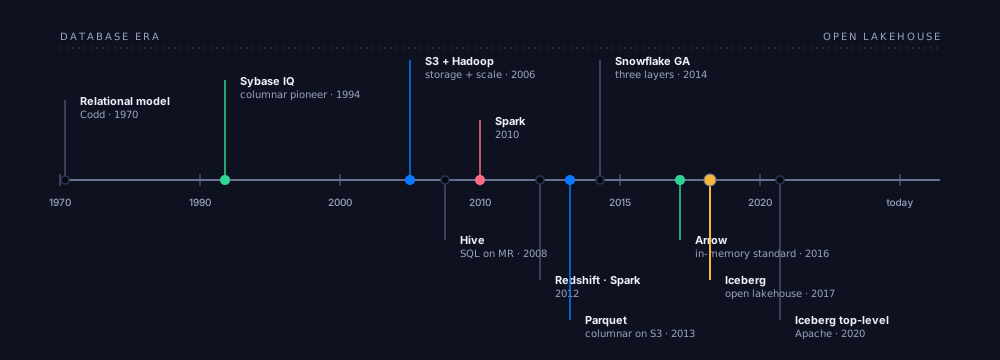
Three things to notice when you lay every event on one axis. First, the warehouse era is long — almost twenty years from Sybase IQ to Snowflake. The architecture wasn't broken; it just needed a different economic regime to evolve. Second, the lake era is dense — Hadoop, Hive, Parquet, and Spark all clustered between 2006 and 2013. Once cheap storage existed, the surrounding ecosystem filled in fast. Third, the table format era is recent — Iceberg, Delta, Hudi all 2016–2017. The lake had been around for a decade by then; the catalog problem was the last piece to be solved.

Each generation pulled one layer apart

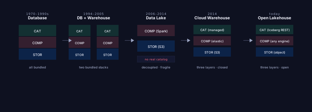
The 1970s rectangle became the 2020s six-layer stack by separating one concern at a time. The warehouse separated analytical from operational. The lake separated storage from compute. Snowflake separated the three commercially. Iceberg separated the table from any one engine. Each move reduced lock-in further. Architecture is rearrangement.

What each generation gave up

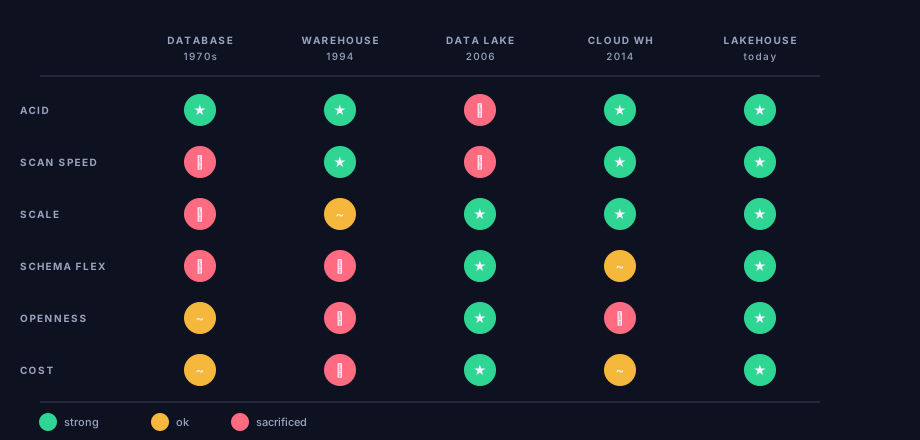
Every era moved some capability up while pushing some other one down. The warehouse won ACID and scan speed but gave up flexibility and cheapness. The lake won scale and openness but gave up transactions and interactivity. The lakehouse column is the first with no big giveaway — and that's not an accident. It's the cumulative payoff of fifty years of trade-off lessons: ACID came back from the warehouse era, scan speed kept the warehouse's strength at lake scale, schema flexibility survived through Iceberg's safe evolution, openness arrived as the organizing principle, and cost came down because storage commoditized.

The lesson is not that the lakehouse is the final answer. It is that the architecture that wins is the one that minimizes the giveaway. Future eras will introduce new constraints — real-time at scale, ML-native data, federated computation across silos — and the answer will preserve what we have here while pushing some new capability up.

Appendix — glossary of recurring terms

A handful of terms recur throughout. Pinned here for reference.

• ACID — Atomicity, Consistency, Isolation, Durability. The contract a database makes about transactions: all-or-nothing writes, always-valid state, transactions don't see each other half-done, committed means permanent.
• OLTP / OLAP — Online Transaction Processing (many small operations, low latency, single rows) versus Online Analytical Processing (fewer queries, each aggregating huge amounts of data).
• MPP — Massively Parallel Processing. Data partitioned across many nodes; a single query runs in parallel across all of them, and results combine.
• Schema-on-write — define the table first, then load data that fits; anything else is rejected. The opposite, schema-on-read, stores data as-is and applies structure at query time.
• Row group — a horizontal slice of a Parquet file (typically 128MB–1GB) inside which each column is stored contiguously. What makes Parquet columnar.
• Predicate pushdown — filtering data as close to storage as possible, using per-row-group min/max statistics to skip data that cannot match.
• Snapshot isolation — each reader sees one consistent snapshot of a table from start to finish, regardless of concurrent writers. Iceberg gives this for free because old snapshots are kept.
• Zero-copy — two processes or languages reading the same memory directly, without transformation. Possible when both agree on the exact byte layout; Arrow's reason for being.
• Vectorized execution — processing data in batches rather than one row at a time, so the CPU's SIMD instructions act on many values at once. The execution model of every modern analytical engine, Dataglot included.
• Federation — querying across multiple data sources from a single engine, without first moving the data into one place.

Appendix — the reference shelf

Original sources for the engineering claims in this essay. Papers over blog posts; primary sources over commentary.

Foundational papers

• Codd — "A Relational Model of Data for Large Shared Data Banks", Communications of the ACM, 1970. The paper that started relational databases.
• Ghemawat, Gobioff, Leung — "The Google File System", SOSP 2003. The architecture that inspired HDFS.
• Dean, Ghemawat — "MapReduce: Simplified Data Processing on Large Clusters", OSDI 2004.
• Stonebraker et al. — "C-Store: A Column-oriented DBMS", VLDB 2005. The academic basis for Vertica and modern column stores.
• Melnik et al. — "Dremel: Interactive Analysis of Web-Scale Datasets", VLDB 2010. Inspired Parquet and BigQuery.
• Zaharia et al. — "Resilient Distributed Datasets", NSDI 2012. Spark's foundational paper.
• Armbrust, Ghodsi, Xin, Zaharia — "Lakehouse Architecture", CIDR 2021. The paper that introduced "lakehouse" as a category.

Open specifications

• Apache Parquet — project home and format spec.
• Apache Iceberg table spec and the Iceberg REST catalog OpenAPI spec.
• Apache Arrow format specification — columnar memory layout, IPC, and Flight.

Engines and catalogs

• Apache DataFusion — the Rust query-execution framework Dataglot credits under the hood.
• Apache Spark, DuckDB — neighboring engines referenced throughout.
• Lakekeeper and Apache Polaris — open Iceberg REST catalog implementations.

Books

• Kleppmann — Designing Data-Intensive Applications (O'Reilly, 2017). The single best book on the architectural concepts in this essay.
• Kimball & Ross — The Data Warehouse Toolkit; Inmon — Building the Data Warehouse. The two original warehouse philosophies.

---

We didn't invent a paradigm. We built cleanly on the one that won.